Description: PIPE Planner paper note — scores frontiers by information gain integrated along the whole A* path rather than at the endpoint, using map predictions to stop pathwise coverage from being overestimated; a polygon-union trick replaces per-step flood fills (83.3% compute cut on large maps) and it reaches 90/95% IoU fastest with zero failures on KTH floor plans
My Notion Note ID: K2E-B-N2-6
Created: 2026-07-19
Updated: 2026-07-19
License: Free to share: please credit Yu Zhang and link back to yuzhang.io

1. Summary

Title: PIPE Planner: Pathwise Information Gain with Map Predictions for Indoor Robot Exploration Authors: S. Baek*, B. Moon*, S. Kim*, M. Cao, C. Ho, S. Scherer†, J. Jeon† (UNIST, Korea; CMU Robotics Institute) — *equal contribution, †equal advising Paper: arXiv:2503.07504 (v2, Aug 2025) Github: castacks/pipe-planner · project page

PIPE (Pathwise Information Gain with Map Prediction for Exploration) — a frontier explorer that evaluates a candidate frontier by the information gathered along the entire path to it, not just at the frontier itself.

Core problem: most exploration planners score information gain pointwise — at the candidate viewpoint only. But real sensors collect data continuously while moving, so pointwise gain understates what a trip actually yields. The obvious fix, pathwise integration, has three problems:

it is computationally expensive (raycast at every point along every candidate path);
it overestimates gain, because rays fly freely through unknown space where undiscovered obstacles would actually block them;
those errors accumulate along the trajectory, compounding into bad decisions.

Key insight: pathwise integration and map prediction fix each other's weaknesses. Integrating along the path captures the true continuous sensing; predicting the map ahead of the robot bounds the raycasts so the accumulated coverage stays realistic. The paper claims to be the first to combine map-prediction-based exploration with a pathwise information-gain metric.

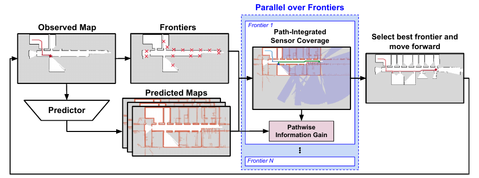
Approach: for each frontier, generate an A* path, probabilistically raycast the predicted map at sampled points along it, merge the per-point visibility polygons into one composite polygon (the key efficiency trick), and sum the ensemble variance inside the resulting mask — normalized by path length.

Main results: on KTH floor plans PIPE has the best IoU area-under-curve at every map size, and is the only method to reach both 90% and 95% IoU with a 0% failure rate across small, medium and large maps. Notably, a pathwise baseline without prediction (PW-NBV-2D) degrades badly as maps grow — evidence that pathwise integration alone is not enough.

PIPE pipeline: frontiers are extracted from the observed occupancy grid while a predictor generates an ensemble of predicted maps; for each frontier (in parallel) the planner computes path-integrated sensor coverage, builds a visibility mask for the full path, and sums the pixelwise prediction variance inside it to get pathwise information gain; the best frontier is selected.

2. Key Contributions

Pathwise information gain with map prediction — path-integrated cumulative sensor coverage combined with predicted maps to suppress overestimation; presented as the first such combination.
Fast expected-observation-mask computation — a computational-geometry formulation (polygon union + hole extraction, one final flood fill) that makes pathwise coverage tractable.
Demonstrated gains over SOTA — PIPE outperforms state-of-the-art indoor exploration baselines on a real-world floor-plan dataset, in both budget-constrained and full exploration.

Beyond those three enumerated contributions, the experiments produce a useful negative result (paper §V-D.3, discussed in §4): a pathwise metric without prediction degrades as maps grow, which isolates prediction as the necessary ingredient.

3. Method

3.1 Problem Setup

2D indoor environment $E \subset \mathbb{R}^2$ ; state $x_t = [x_t, y_t]$ with integer coordinates; a noise-free 2D LiDAR of range $\lambda$ collecting $l$ evenly distributed samples over $360^\circ$ . The robot maintains an occupancy grid $O_t$ (free / occupied / unknown) and moves a step $\Delta$ per timestep on an 8-connected grid. Goal: a feasible path $\{x_0, \dots, x_T\}$ that builds an accurate map within budget $T$ .

Framework is classical frontier-based exploration, upgraded from "nearest frontier" to a next-best-view style rule driven by the information-gain metric below. A predicted map $M_t$ comes from a pretrained inpainting network (LaMa) applied to $O_t$ , and an uncertainty map $U_t$ is the pixelwise variance across an ensemble of predictions. The distinguishing choice: the robot selects the holistic next best frontier, scoring the path to it rather than the frontier observation alone.

3.2 Sensor Coverage & Visibility Masks

Coverage at a state is estimated by raycasting:

\{v_{1:l}\} \leftarrow \textsc{Raycast}(f, \lambda, M_t), \qquad G \leftarrow \textsc{DrawPolygon}(\{v_{1:l}\}), \qquad \nu \leftarrow \textsc{FloodFill}(G)

$\{v_{1:l}\}$ = the vertices where the $l$ rays terminate, $G$ = the polygon they bound, $\nu$ = the filled visibility mask (estimated sensor coverage). Raycasting on $M_t$ rather than $O_t$ is what lets the robot reason beyond what it has seen.

Probabilistic raycast (adopted from MapEx): stopping a ray at the first predicted-occupied cell underestimates coverage when the predictor wrongly marks free space as occupied. Instead each ray accumulates traversed cell values into $\delta$ (from $\delta = 0$ ) and stops once $\delta$ reaches threshold $\epsilon$ ; tuning $\epsilon$ trades over- against under-estimation. PIPE follows prior work with $\epsilon = 0.8$ .

3.3 Path-Integrated Sensor Coverage

For each frontier $f_i \in F$ , build an A* path $P_i$ from the current pose $x_t$ to $f_i$ , and sample points $p_j$ along it every $\Delta$ (the same spacing as one robot timestep, so the samples match where the robot would actually sense). Raycast at each $p_j$ on $M_t$ :

\{v_{1:l}\}_j \leftarrow \textsc{Raycast}(p_j, \lambda, M_t), \quad G_j \leftarrow \textsc{DrawPolygon}(\{v_{1:l}\}_j), \quad \nu_j \leftarrow \textsc{FloodFill}(G_j)

The path-integrated coverage is the union of the per-point masks $\nu_j$ . Done naively this is prohibitively slow.

3.4 Making It Fast

Where the time goes: profiling on small/medium/large KTH maps showed frontier evaluation consumes 80.9% / 93.7% / 97.3% of total compute (the share grows with map size as frontier count and path length grow), and within that, visibility-mask generation dominates — the repeated flood fills are the bottleneck.

The trick: don't flood-fill each polygon. First merge, then fill once. Because unioned raycast polygons are usually non-convex, the union can enclose holes (trapped regions) that must not be filled, so they are recovered via symmetric difference:

G_{\text{union}} = \bigcup_j G_j, \qquad S = \bigcup_j \left( G_j \,\triangle\, G_{\text{union}} \right), \qquad H = S \setminus G_{\text{union}}, \qquad \nu = \textsc{FloodFill}(G_{\text{union}}, H)

$\triangle$ = symmetric difference, $H$ = the set of holes, $\nu$ = final path visibility mask. Deferring the one expensive flood fill to the merged polygon is the main saving. On top of that, frontiers are evaluated in parallel across CPU cores (Python multiprocessing), ideally scaling with core count.

Combined, the optimizations cut computation by 83.3% on large maps (measured on an Intel Core i5-10400F / RTX 3060 / 16 GB desktop).

3.5 The PIPE Planner

Per waypoint decision: extract frontiers $F$ from $O_t$ ; generate ensemble predictions $M_t$ and variance $U_t$ ; then for each frontier $f$ — A* path $P$ , path visibility mask $\nu$ , and

I = \sum_{(x_k, y_k) \in \nu} U_t(x_k, y_k), \qquad \text{score}(f) = \frac{I}{\lvert P \rvert}

$I$ = pathwise information gain (uncertainty observed along the whole path), $\lvert P \rvert$ = path length. Normalizing by path length (rather than Euclidean distance, as in pointwise methods) keeps the metric consistent with the path-integrated numerator. The argmax frontier becomes the waypoint; the robot follows an A* path and re-plans on arrival.

4. Experiments & Results

Setup: custom simulator over the KTH floor-plan dataset (>100 campus floor plans as XML wall/door descriptions), maps corrected for raycast-breaking inaccuracies and downsampled to 10 pixels/m. Seven floor plans in three size classes — 2 small (65 × 85 m), 3 medium (60 × 205 m), 2 large (88 × 265 m) — each run from 25 distinct start locations, for 175 experiments total. Map predictions from LaMa.

Metric: IoU of occupied cells between predicted and ground-truth maps, $\text{IoU} = \tfrac{TP}{FP+FN+TP}$ , with a small buffer so that sub-pixel misalignment isn't penalized. Methods without a predictor (NBV-2D, PW-NBV-2D, Nearest) have predicted maps generated post-hoc from their observed maps so the comparison is apples-to-apples.

Baselines, spanning the pointwise/pathwise × prediction/no-prediction design space:

Method	Pointwise / Pathwise	Prediction	Gain signal
Nearest	—	no	Euclidean distance only
NBV-2D	pointwise	no	sensor coverage on $O_t$
PW-NBV-2D	pathwise	no	sensor coverage on $O_t$
UPEN	pathwise	yes	uncertainty only (no coverage)
MapEx	pointwise	yes	coverage + uncertainty
PIPE	pathwise	yes	coverage + uncertainty

IoU area-under-curve (higher is better):

Method	Small	Medium	Large
PIPE	327.00	648.35	1338.16
MapEx	290.63	607.05	1278.39
PW-NBV-2D	316.81	587.59	1184.69
NBV-2D	295.68	582.70	1209.37
UPEN	270.04	494.08	1084.57
Nearest	244.80	482.79	971.30

PIPE leads at every size, though the runner-up changes: PW-NBV-2D is second on small maps, MapEx on medium/large.

Complete exploration — timesteps to reach 90% / 95% IoU (max 1500 / 3000 / 6000 steps for small / medium / large; FR = failure rate, runs not reaching the target):

Method	Small 90%	Medium 90%	Large 90%	FR at 95% (S/M/L)
PIPE	505 ± 41	1039 ± 56	1979 ± 115	0 / 0 / 0
MapEx	610 ± 38	1165 ± 72	2266 ± 164	0 / 3 / 2
PW-NBV-2D	519 ± 40	1643 ± 146	3732 ± 243	12 / 51 / 32
NBV-2D	577 ± 34	1321 ± 65	2336 ± 89	0 / 4 / 0
UPEN	833 ± 85	2171 ± 168	4085 ± 301	64 / 63 / 62
Nearest	1050 ± 57	2273 ± 77	4109 ± 249	12 / 33 / 4

PIPE needs the fewest steps everywhere and is the only method that never fails to complete at either threshold.

The interesting negative result: PW-NBV-2D (pathwise, no prediction) is competitive on small maps but collapses on large ones — 15.20% behind PIPE there, a much wider gap than at small scale. Without a predicted map, its rays fly unobstructed through unknown space and it badly overestimates cumulative coverage; the error compounds with path length. So pathwise integration alone is insufficient — it can even hurt unless paired with prediction. Conversely the pointwise methods (NBV-2D, MapEx) tend to fixate on one region of the map, showing the short-sightedness that pathwise reasoning fixes.

5. Strengths / Limitations / Future Work

Strengths

Fixes a genuine mismatch: sensors gather data continuously, so scoring only the endpoint is the wrong model.
The efficiency contribution is real engineering, not an afterthought — profiling identified flood fill as the bottleneck and the polygon-union reformulation removes it (83.3% cut on large maps), turning an infeasible metric into a practical one.
Honest, well-designed baseline grid that isolates both axes (pointwise↔pathwise, prediction↔none), producing the informative negative result about PW-NBV-2D.
Strong reliability story: zero failure rate is arguably more compelling than the IoU margins.

Limitations

Same idealizations as MapEx: 2D, noise-free LiDAR, implicitly known pose — no SLAM drift or 3D structure; simulation only, no real-robot deployment.
On large maps the IoU margin over MapEx/NBV-2D is modest (≈2–5%); the clearer wins are in completion time and failure rate.
Still depends on a predictor fine-tuned on the same KTH floor-plan style — generalization to unfamiliar building layouts is untested.
Parallelism relies on CPU cores; per-frontier A* plus ensemble prediction each replan is still heavier than pointwise scoring.
$\epsilon = 0.8$ is inherited rather than re-tuned, and path-length normalization remains a heuristic trade-off between gain and travel cost.

Future work (note-level extrapolation, not stated by the paper): 3D / real-robot validation with pose and range noise, multi-robot pathwise coordination, and learning the predictor jointly with the planning objective.

References

Baek, S., Moon, B., Kim, S., Cao, M., Ho, C., Scherer, S., & Jeon, J. (2025). PIPE Planner: Pathwise Information Gain with Map Predictions for Indoor Robot Exploration. arXiv:2503.07504, code. — source paper (Fig. 2 pipeline diagram above)
MapEx: the pointwise predecessor from the same group — PIPE adopts its probabilistic raycast, and follows both MapEx and UPEN for the ensemble-variance uncertainty map. MapEx is the strongest baseline on medium and large maps (on small maps PW-NBV-2D edges it out)
Yamauchi, B. (1997). A Frontier-Based Approach for Autonomous Exploration. IEEE CIRA. — the Nearest baseline
Georgakis, G., et al. (2022). Uncertainty-driven Planner for Exploration and Navigation (UPEN). ICRA. — pathwise, uncertainty-only baseline
Bircher, A., et al. (2016). Receding Horizon Next-Best-View Planner for 3D Exploration. ICRA. — the next-best-view paradigm the NBV-2D baselines descend from
Liu, J., Wang, C., Chi, W., Chen, G., & Sun, L. (2022). Estimated Path Information Gain-Based Robot Exploration under Perceptual Uncertainty. Robotica, 40(8). — closest prior pathwise-coverage work; approximates cumulative coverage with parallelograms
Suvorov, R., et al. (2022). Resolution-robust Large Mask Inpainting with Fourier Convolutions (LaMa). WACV. — the map predictor

Table of Contents